EvAM-Tools
Table of contents
- EvAM-Tools
- A two-paragraph summary about cross-sectional data and EvAMs (or CPMs)
- What EvAMs are included inEvAM-Tools? - User’s Manual: How to use this web interface?
- Web app: overview of workflow and functionality
-User input
- Analyze data:Run evamtools
-Results
- Default options and default EvAMs run
- Example files for upload
- How long does it take to run?
- Session timeouts, RAM and elapsed time execution limits, aborting a run
- Additional documentation - References and related repositories
- Where is the code? Terms of use. Citing. Copyright
- Authors, contact and bug reports
- Citing EvAM-Tools - Funding
- Cookies
EvAM-Tools
EvAM-Tools is an R package and Shiny web app that provides tools for evolutionary accumulation models (EvAMs). We use code from “Cancer Progression Models” (CPMs) but these are not limited to cancer (the key idea is that events are gained one by one, but not lost). EvAM-Tools is also available as an R package (see https://github.com/rdiaz02/EvAM-Tools).
This Shiny web interface provides a GUI to the package and focuses on allowing fast construction, manipulation, and exploration of EvAM/CPM models, and making it easy to gain an intuitive understanding of what these methods infer from different data sets as well as what kind of data are to be expected under these models. You can analyze your data, create cross-sectional data from scratch (by giving genotype frequencies), or generate synthetic data under different EvAMs/CPMs. You can compare results from different methods/models, as well as experiment and understand the consequences of changes in the input data on the returned inferences. You can also examine how a given method performs when data have been generated under another (or its own) model.
This landing page is the main documentation for the use of the web interface. Additional examples of use are discussed in https://github.com/rdiaz02/EvAM-Tools#some-examples-of-use and in the “EvAM-Tools: examples” additional documentation file (though they do not —yet— include HyperTraPS-CT nor BML). The R package itself contains documentation using standard R mechanisms, and gives you access to some additional functionality not exposed via the web app.
New as of May 2025: We have added two new methods: HyperTraPS-CT and BML.
Funding: Supported by grant PID2019-111256RB-I00 funded by MCIN/AEI/10.13039/501100011033 and Comunidad de Madrid’s PEJ-2019-AI/BMD-13961 to R. Diaz-Uriarte.

A two-paragraph summary about cross-sectional data and EvAMs (or CPMs)
In cross-sectional data a single sample is obtained from each subject or patient. That single sample represents the “observed genotype” of, for example, the tumor of that patient. Genotype can refer to single point mutations, insertions, deletions, or any other genetic modification. In this app, as is often done by EvAM software, we store cross-sectional data in a matrix, where rows are patients or subjects, and columns are genes; the data is a 1 if the event was observed and 0 if it was not.
Cancer progression models (CPMs) or, more generally, evolutionary accumulation models (EvAMs), use these cross-sectional data to try to infer restrictions in the order of accumulation of events; for example, that a mutation on gene B is always preceded by a mutation in gene A (maybe because mutating B when A is not mutated). Some cancer progression models, such as MHN, instead of modeling deterministic restrictions, model facilitating/inhibiting interactions between genes, for example that having a mutation in gene A makes it very likely to gain a mutation in gene B. A longer explanation is provided in What EvAMs are included in EvAM-Tools?, below, and many more details in EvAM-Tools: methods’ details and FAQ. Finally, note we have talked about “genotype” and “mutation”, but EvAMs have been used with non-genetic data too, and thus our preference for the expression “event accumulation models”; as said above, the key idea is that events are gained one by one, but not lost, and that we can consider the different subjects/patients in the cross-sectional data as replicate evolutionary experiments or runs where all individuals are under the same constraints (e.g., genetic constraints if we are dealing with mutations).
What EvAMs are included in EvAM-Tools?
-
Oncogenetic Trees (OT): Restrictions in the accumulation of mutations (or events) are represented as a tree. Hence, a parent node can have many children, but children have a single parent. OTs are untimed (edge weights represent conditional probabilities of observing a given mutation, when the sample is taken, given the parents are observed).
-
Conjuntive Bayesian Networks (CBN): This model generalizes the tree-based restriction of OT to a directed acyclic graph (DAG). A node can have multiple parents, and it denotes that all of the parents have to be present for the children to appear. Therefore, relationships are conjuntive (AND relationships between the parents). These are timed models, and the parameters of the models are rates given that all parents have been observed. We include both H-CBN as well as MC-CBN.
-
Hidden Extended Suppes-Bayes Causal Networks (H-ESBCN): Somewhat similar to CBN, but it includes automatic detection of logical formulas AND, OR, and XOR. H-ESBCN is used by its authors as part of Progression Models of Cancer Evolution (PMCE). Like CBN, it returns rates.
-
OncoBN: Similar to OT, in the sense of being an untimed oncogenetic model, but allows both AND (the conjunctive or CBN model) and OR relationships (the disjunctive or DBN model).
-
Mutual Hazard networks (MHN): With MHN dependencies are not deterministic and events can make other events more like or less likely (inhibiting influence). The fitted parameters are multiplicative hazards that represent how one event influences other events.
-
Hypercubic transition path sampling (HyperTraPS-CT): HyperTraPS-CT is also a stochastic dependencies model, like MHN, where events can have an inhibiting or promoting effect on other events. HyperTraPS-CT can use models with pairwise interactions between events, like MHN, but also models of lower-order (no interactions between events) and higher-order interactions (three-way, four-way, and full parameterisation —set this with the “model” argument). For the cross-sectional data we use here, HyperTraPS-CT uses discrete-time modelling, but HyperTraPS-CT also supports continuous time models as well as phylogenetically- and longitudinally-related samples, but this is not —yet— available via the Shiny app.
-
Bayesian Mutation Landscape (BML): tries to reconstruct evolutionary progression paths and ancestral genotypes. It can highlight epistatic interactions between genes.
For details, please see the EvAM-Tools: methods’ details and FAQ; see also the review paper Diaz-Uriarte, R., & Johnston, I. G. (2025), https://doi.org/10.1109/ACCESS.2025.3558392 .
User’s manual: How to use this web interface?
Web app: overview of workflow and functionality
The figure below provides an overview of the major workflows with the web app (that figure does not include HyperTraPS nor BML, but the workflow is similar for those methods):
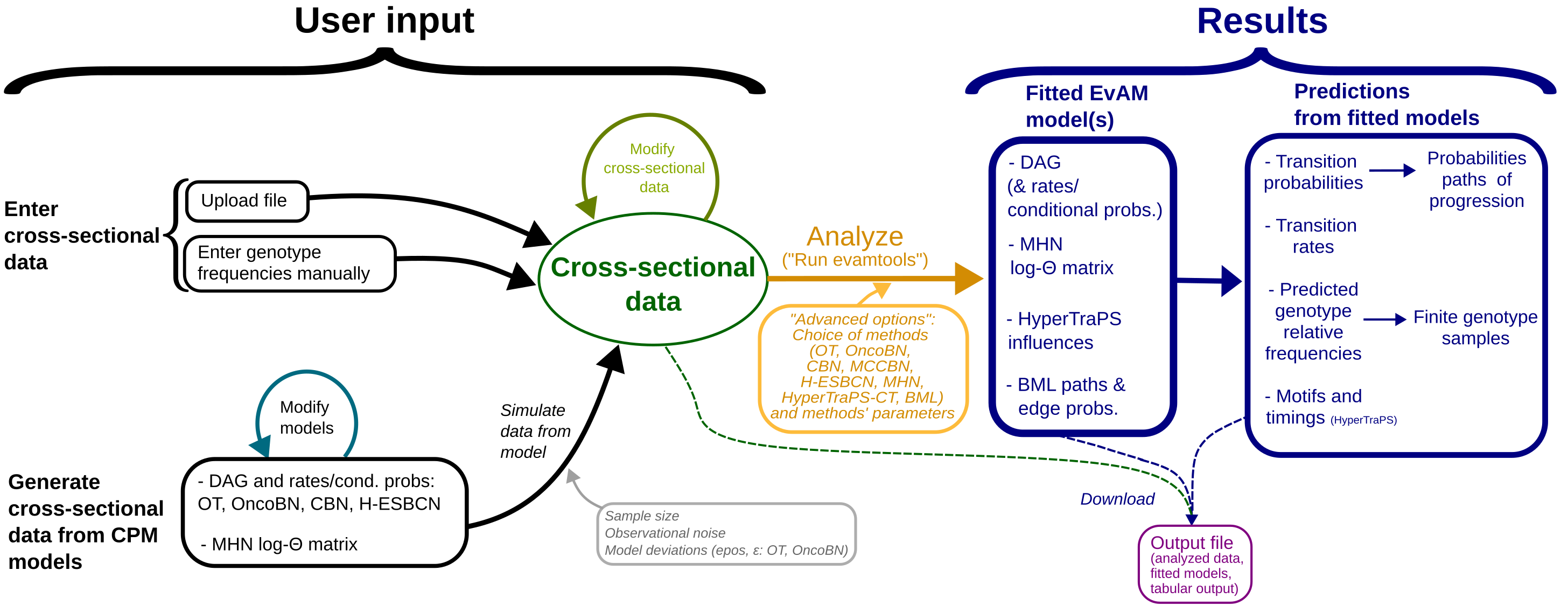
The web app encompasses, thus, different major functionalities and workflows, mainly:
-
Inference of EvAMs from user data uploaded from a file.
-
Exploration of the inferences that different EvAM methods yield from manually constructed synthetic data.
-
Construction of EvAM models (DAGs with their rates/probabilities and MHN models) and simulation of synthetic data from them.
3.1. Examination of the consequences of different EvAM models and their parameters on the simulated data.
3.2. Analysis of data simulated under one model with methods that have different models (e.g., data simulated from CBN analyzed with OT and OncoBN).
3.3. Analysis of data simulated under one model with manual modification of specific genotype frequencies prior to analyses (e.g., data simulated under CBN but where, prior to analysis, we remove all observations with the WT genotype and the genotype with all loci mutated).
Furthermore, note that in all cases, when data are analyzed, in addition to returning the fitted models, the web app also returns the analysis of the EvAMs in terms of their predictions such as predicted genotype frequencies and transition probabilities between genotypes.
The figure below highlights the different major functionalities and workflows, as numbered above, over-imposed on the previous figure:

We explain now in more detail the functionality, options, input, and output, of the web app. Commented examples that illustrate each of those workflows are provided in the EvAM-Tools: examples additional documentation file.
User input
To start using the web app, go first to the User input tab (on top of the page). Here you can:
- Enter cross-sectional data directly by either:
- Uploading a file.
- Entering genotype frequencies manually
- Generate cross-sectional data from EvAM models. Follow these steps:
-
Specify the EvAM model first. You can use:
1.1. Models that use DAGs to specify restrictions: OT, OncoBN (in both its conjunctive and disjunctive versions), CBN and H-ESBCN (H-ESBCN allows you to model AND, OR, and XOR dependency relationships). You will specify the DAG and the rates (CBN, H-ESBCN)/conditional probabilities (OT, OncoBN) of events conditional on their parents.
1.2. MHN, that models inhibiting/facilitating relationships between genes using baseline hazard rates and multiplicative effects between genes (specified in the log-Θ matrix).
(1.3. This is not available for HyperTraPS or BML.)
-
Simulate data from the EvAM model. In addition to the number of samples, you can specify the amount of observational noise (and, for OT and OncoBN, deviations from the model).
Note that simulating data from EvAMs allows you to get an intuitive feeling for what different EvAM models and their parameters mean in terms of the genotype frequency data they produce.
-
Cross-sectional data that have been uploaded or simulated from EvAM models can be further modified by altering genotype counts. Moreover, it is possible to specify cross-sectional data and DAG/MHN models with user-specified gene names. Finally, from the “User input” tab you can also save the cross-sectional data.
To make it easier to play with the tool, we provide predefined cross-sectional data sets under “Enter genotype frequencies manually”, as well as predefined DAG and MHN models (from which you can generate data by clicking on “Generate data from DAG [MHN model]”). You can also modify the predefined DAGs and MHNs before generating data.
Analyze data: Run evamtools
- Change, if you want, the options under “Advanced options and EvAMs to use” (on the right of the screen). These options include what EvAM methods to use as well as parameters of the methods.
- Click on “Run evamtools”.
- Results will be shown in the
Resultstab.
Results
The results include:
-
The fitted EvAMs (or CPMs) themselves, including the DAGs with their rates/conditional probabilities (depending on the model) and the MHN log-Θ matrix.
-
Predictions derived from the fitted models, including:
-
Transition probabilities: conditional probability of transition to a genotype (obtained using competing exponentials from the transition rate matrix for all methods except OT and OncoBN). For OT and OncoBN this is actually an abuse of the untimed oncogenetic tree model; see the Evamtools: methods’ details and FAQ for details.
-
Transition rates: for models that provide them (CBN, H-ESBCN, MHN) transition rates of the continuous-time Markov chain that models the transition from one genotype to another. This option is not available for OT and OncoBN, as these do not return rates.
-
Predicted genotype relative frequencies: the predicted genotype frequencies from the fitted models.
The predicted genotype frequencies for CBN, HESBCN and MHN are obtained assuming sampling time is exponentially distributed with rate 1.
For OncoBN and OT, the predicted frequency of genotypes corresponds to the predicted frequency on the sample collection (these are untimed models, and sampling time is not assumed to follow any specific distribution).
For HyperTraPS, we we use function
state.probs, which returns P(state | probability that n features have been acquired = P_n). If you use the default value ofprob.set(underAdvanced options),observed, we set P_n to the value observed in the input sample (i.e., P_0 = the proportion of observations with 0 mutations in the input sample, P_1 = the proportion of observations with 1 mutation in the input sample, etc). If you useNA, we set P_n = 1/(L+1)), i.e., the sampling model is one where the probability of acquiring 0, 1, …, features is the same. You can specify a different sampling scheme by modifyingprob.setand passing a vector of probabilities for 0, 1, …, features. -
Sampled genotype counts: Counts, or absolute genotype frequencies obtained by generating a finite sample (of the size you chose) with the probabilities given by the predicted genotype frequencies. If you add noise, the sampled genotype counts include observational (e.g., genotyping) noise. (To generate sampled genotype counts, you have to select the option from “Advanced options”, as this is disabled by default.)
-
Note that not all predictions are available for all methods. (No transition rate matrices are available for OT and OncoBN, since those are untimed models; HyperTraPS does not give as output transition rate matrices per se; BML does not provide transition matrices nor transition rate matrices nor predicted genotype frequencies.)
-
The results are displayed using a combination of figures and tabular output. Specifically:
-
The first row of figures shows the fitted EvAMs: DAGs with their rates/probabilities and MHN log-Θ matrix.
-
The edges of the DAGs are annotated with the lambda (CBN, HESBCN), weight (OT) or θ (OncoBN).
-
Remember: for DAGs, these are DAGs that have genes (not genotypes) as nodes. They represent the order restrictions of the events.
-
For MHN there is no DAG of restrictions; we show the fitted log-Θ matrix rounded to two decimal places. The diagonal entries are the log-baseline rates, and the off-diagonal the log of the multiplicative effects of the effector event (the columns) on the affected event (rows).
-
You can represent the results of all the fitted models or only of a subset (select those using “EvAMs to show”).
-
For HyperTraPS the output in the first row depends on the model. For models with pairwise interactions (
model = 2), we show the pairwise influences between features (this is similar to the output from MHN), calling hypertraps’ packageplotHypercube.influencesfunction. For models with 3-way interactions (model = 3) we show “how each feature acquisition influences the rate of acquisition of other features as a network” (from https://github.com/StochasticBiology/hypertraps-ct/tree/bioconductor#visualising-and-using-output), calling hypertraps’ packageplotHypercube.influencegraphfunction. In both cases, if you used regularisation, the output shows the parameters from the regularised model. For other models (unrestricted —model = -1—, main-effects only —model = 1—, and four-way interactions —model = 4—), we show a “motif plot of feature acquisition probabilities at discrete orderings”, calling hypertraps’ packageplotHypercube.motifsfunction. -
For BML, we do not show DAGs of restrictions (nor matrices as for MHN and HyperTraPS), since BML does not return these. Instead, we show plots as in Fig. 2 of Misra et al., 2014. These plots show the most likely paths of progression. As explained in that paper (p. 2460, legend Fig. 2) “Color for a genotype g with k mutations is scaled according to its relative probability P(g)/mk (decreasing from darker shade to light), where mk is the maximum probability for a node with k mutations (Section 3).” [As explained in pp. 2456 and ff., P(g) is the probability “that a particular combination of mutations (denoted by genotype g) reaches fixation in a cell population that has evolved from a normal cell genotype and will eventually attain a tumor cell genotype. (…) [it is] the evolutionary probability of genotype g. P(g) equals the sum of path probabilities for every mutation path from the normal genotype that passes through g and ends as atumor genotype.”]
-
- The second row of figures shows the predictions derived from the fitted models. These same predictions are also displayed in tabular output on the bottom right. On the left side panel (“Customize the visualization”), you choose what predictions you want to display. Not all predictions are available for all methods (e.g., none of them are available for BML; transition rate matrices are not available for OncoBN or OT, nor as such for HyperTraPS). Note that for HyperTraPS, the transition matrix shown here is showing the same information as shown by the hypercube graph shown in the summary figures underneath.
- The plots that show Transition probabilities and Transition rates (again, on the second row of figures) have genotypes (not genes) as nodes.
- You can show, for these transition plots, only some of the most relevant paths; again, modify options under “Customize the visualization”.
- These plots might include genotypes never observed in the sample; these are shown in light green.
- For easier visualization, in very busy plots, instead of the Genotypes you might want to show the last gene (or event) mutated or gained; change this options under “Type of label”.
- (As visualizing the acquisition of mutations in a complex network can be challenging, for the transition probabilities/rates plots we use the representation of the hypergraph transition graph from HyperTraPS — Greenbury et al., 2020. HyperTraPS: Inferring probabilistic patterns of trait acquisition in evolutionary and disease progression pathways. Cell systems, 10, 39–51, https://doi.org/10.1016/j.cels.2019.10.009)
- For HyperTraPS, we show summary plots as provided by a custom modification of hypertraps’ package
plotHypercube.summaryfunction. The plots provided are, from left to right and from top to bottom:- A trace of the likelihood (“re-calculated twice with different samples (to show consistency or lack thereof), along with current ‘in use’ likelihood” [the current ‘in use’ or ‘working’ likelihood is the red line] —from https://github.com/StochasticBiology/hypertraps-ct/tree/bioconductor#visualising-and-using-output).
Using the likelihood trace to assess performance is discussed in the README, section “Assessing performance”.
Examples illustrating issues with estimation and chains, that can be detected from the likelihood trace, are available from Example 6 of file hypertraps-demos.R (link to actual line here). That same file
hypertraps-demos.R(https://github.com/StochasticBiology/hypertraps-ct/blob/bioconductor/demos/hypertraps-demos.R#L70) contains guidance on the use of the likelihood traces, that we copy verbatim with minor edits: “Examine the likelihood traces. These should show:- Overlap between dashed black and red lines. If not, likelihood estimates aren't converging; use more random walkers. [increase the value of the "walkers" option]
- Constant mean likelihood (no systematic up or down). If not, MCMC chain isn't converged; use run longer chains. [increase the value of the "length" option]
- Uncorrelated (white) noise; no periods of stasis. If not, MCMC chain is getting stuck; use a smaller kernel. [decrease the value of the "kernel" option]"
- A “‘Bubble plot’ of probability of acquiring trait i at ordinal step j”.
- “Transition graph with edge weights showing probability flux (from sampled paths).” This is very similar to the “Transition probabilities” plot on the second row.
- A “motif plot of feature acquisition probabilities at discrete orderings”, calling hypertraps’ package
plotHypercube.motifsfunction. (If you used a model different from 2 or 3, you will also see this plot in the first row.) - See https://github.com/StochasticBiology/hypertraps-ct/tree/bioconductor#visualising-and-using-output for details.
- A trace of the likelihood (“re-calculated twice with different samples (to show consistency or lack thereof), along with current ‘in use’ likelihood” [the current ‘in use’ or ‘working’ likelihood is the red line] —from https://github.com/StochasticBiology/hypertraps-ct/tree/bioconductor#visualising-and-using-output).
Using the likelihood trace to assess performance is discussed in the README, section “Assessing performance”.
Examples illustrating issues with estimation and chains, that can be detected from the likelihood trace, are available from Example 6 of file hypertraps-demos.R (link to actual line here). That same file
- For BML, if you used bootstrap, we show plots like Fig. 3a and 3b of Misra et al. 2014:
- On the left, similar to Fig 3a, we plot “Edge probabilities”; from the “README.txt” file of the original code (https://bml.molgen.mpg.de/ ) “[this figure shows] the evolutionary probabilities and departures from independence (multiplicative for P(g), additive for logP(g)) for each pair of genes that had an edge between them in the inferred Bayes net. Each edge is associated with 4 rows, two for the probability of each gene being mutated all by itself, a third row for the pair of genes being mutated and a fourth for the estimate in the absence of correlation for the mutation probabilities.” We color the probability of each gene by itself in red, the pair in blue and the estimate in the absence of correlation in gray.
- On the right, similar to Fig 3b in Misra et al. 2014, we plot “Tree_OBS_Probabilities”: “the evolutionary probabilities for the top ordered genes during OBS [ordering-based search] for each bootstrap replicate using the tree based search. Each row gives the probability for a given gene being mutated and all other genes being normal.”
To help interpret the results, we also show a histogram of the genotype counts of the analyzed data.
Finally, you can also download the tabular results, fitted models, and the analyzed data. To download figures, either use screen captures or use your web browser to download them (e.g., right click on a figure to obtain a menu with a “Save image as” entry —if you need higher resolution or original PDF images, you will need to use the R package itself).
Default options and default EvAMs run
- In the Shiny app, by default we run CBN, OT, OncoBN, MHN, and HyperTraPS. If you want to run H-ESBCN, MC-CBN, or BML, or not run some of the above methods, (de)select them under
Advanced options and EvAMs to use. (H-ESBCN or MC-CBN are not run by default, as they can take a long time). - OncoBN can be run using a conjunctive or a disjunctive model. The default used in the Shiny app (and the
evamfunction in the package) is the disjunctive model. You can use the conjunctive one by selecting it underAdvanced options and EvAMs to use, inOncoBN options,Model. - Most methods have other options that can be modified. Again, check
Advanced options and EvAMs to use.
Example files for upload
In https://github.com/rdiaz02/EvAM-Tools/tree/main/examples_for_upload there are several files in CSV format ready to be used as examples for upload. The two files mentioned in the documentation are: ov2.csv and BRCA_ba_s.csv.
How long does it take to run?
It depends on the number of genes or features and methods used. For six genes, and if you do not use H-ESBCN nor MC-CBN, it should take about 20 seconds. If you do not use CBN either (i.e., if you only use MHN, OT, and OncoBN) it should run in less than 8 seconds. Model fitting itself is parallelized, but other parts of the program cannot be (e.g., displaying the final figures).
Session timeouts, RAM and elapsed time execution limits, aborting a run, reporting crashes
-
Timeouts: Inactive connections will timeout after 2 hours. The page will become gray, and if you refresh (e.g., F5 in most browsers) after this time, you will not get back your results, figures, etc, but start another session.
-
RAM and time limits: Maximum RAM of any process is limited to 4 GB. Likewise, the analyses should be aborted after 1.5 hours of elapsed (not CPU —we parallelize the runs) time. If you want to use the Shiny app without these limits, install a local copy. (To modify the time limit, change the value of variable EVAM_MAX_ELAPSED, in the definition of function “server”, in file “server.R”. The RAM limit is imposed on the Docker containers we use; to remove it, run Docker without the memory limit.) Note: because of the way we enforce these limits, running over limits might not be signalled by an explicit error, but rather by a graying out or a complete refresh of the session.
-
Aborting a run: Sometimes you might want to abort a run (e.g., you might have accidentally sent a run that will take a very long time). This is not possible if you run in our servers. What if you do not care about the long running, not-yet-fished run, and want to start a new one? If, from the same computer and browser, you open a new tab to https://iib.uam.es/evamtools it is very likely that the request will be served by the exact same session and docker process as the previous run; thus, if R has not finished running, you would have to wait for the previous session to finish (and even connecting to a Shiny session might not work).
To continue using EvAM-Tools you can try one or more of these:
- Force a refresh or reload of the page (e.g., “Ctrl + Shift + r”, “Ctrl + F5”).
- Close the browser, and open it again.
- Start a new connection from a different web browser.
- Start a new connection from an incognito session of the same web browser.
- (Note: some of the above, with some browsers, can return a “Proxy error” message. This is due to time outs: until the busy shiny/R process is not done, the connection to that very shiny/R process might fail. Just use a different web browser.)
- Use a different computer.
None of those will abort the old process; that old process will eventually finish or be aborted. But you will be able to continue using EvAM-Tools. (That said, please make considerate use of this service: it is provided free of charge, so do not abuse it.)
-
Crashes: Sometimes, the R process might crash (e.g., a segfault). If this happens, you will most likely only see a graying out of the page. If this happens, please let us know (solving this is complicated, because we have not been able to reliably generate these crashes), giving as much detail as possible.
Additional documentation
Additional documents are available from https://rdiaz02.github.io/EvAM-Tools .
For users of the web app, the most relevant are: EvAM-Tools: examples and EvAM-Tools: methods’ details and FAQ.
References and related repositories
Overview paper on CPMs and EvAMs
- Diaz-Uriarte, R., & Johnston, I. G. (2025). A picture guide to cancer progression and evolutionary accumulation models: Systematic critique, plausible interpretations, and alternative uses. Ieee Access, 13, 62306–62340. https://doi.org/10.1109/ACCESS.2025.3558392
OT
-
Desper, R., Jiang, F., Kallioniemi, O. P., Moch, H., Papadimitriou, C. H., & Sch"affer, A A (1999). Inferring tree models for oncogenesis from comparative genome hybridization data. J Comput Biol, 6(1), 37–51.
-
Szabo, A., & Boucher, K. M. (2008). Oncogenetic Trees. In W. Tan, & L. Hanin (Eds.), Handbook of Cancer Models with Applications (pp. 1–24). : World Scientific. https://doi.org/10.1142/9789812779489_0001
-
Oncotree R package: https://CRAN.R-project.org/package=Oncotree
H-CBN and MC-CBN
-
Beerenwinkel, N., & Sullivant, S. (2009). Markov models for accumulating mutations. Biometrika, 96(3), 645.
-
Gerstung, M., Baudis, M., Moch, H., & Beerenwinkel, N. (2009). Quantifying cancer progression with conjunctive Bayesian networks. Bioinformatics, 25(21), 2809–2815. http://dx.doi.org/10.1093/bioinformatics/btp505
-
Gerstung, M., Eriksson, N., Lin, J., Vogelstein, B., & Beerenwinkel, N. (2011). The Temporal Order of Genetic and Pathway Alterations in Tumorigenesis. PLoS ONE, 6(11), 27136. http://dx.doi.org/10.1371/journal.pone.0027136
-
Montazeri, H., Kuipers, J., Kouyos, R., B"oni, J"urg, Yerly, S., Klimkait, T., Aubert, V., … (2016). Large-scale inference of conjunctive Bayesian networks. Bioinformatics, 32(17), 727–735. http://dx.doi.org/10.1093/bioinformatics/btw459
-
GitHub repository for MC-CBN: https://github.com/cbg-ethz/MC-CBN
-
Source code for h/ct-cbn: https://bsse.ethz.ch/cbg/software/ct-cbn.html
MHN
-
Schill, R., Solbrig, S., Wettig, T., & Spang, R. (2020). Modelling cancer progression using Mutual Hazard Networks. Bioinformatics, 36(1), 241–249. http://dx.doi.org/10.1093/bioinformatics/btz513
-
GitHub repository: https://github.com/RudiSchill/MHN
H-ESBCN (PMCE)
-
Angaroni, F., Chen, K., Damiani, C., Caravagna, G., Graudenzi, A., & Ramazzotti, D. (2021). PMCE: efficient inference of expressive models of cancer evolution with high prognostic power. Bioinformatics, 38(3), 754–762. http://dx.doi.org/10.1093/bioinformatics/btab717
-
Repositories and terminology: we will often refer to H-ESBCN, as that is the program we use, as shown here: https://github.com/danro9685/HESBCN. H-ESBCN is part of the PMCE procedure: https://github.com/BIMIB-DISCo/PMCE.
OncoBN (DBN)
-
Nicol, P. B., Coombes, K. R., Deaver, C., Chkrebtii, O., Paul, S., Toland, A. E., & Asiaee, A. (2021). Oncogenetic network estimation with disjunctive Bayesian networks. Computational and Systems Oncology, 1(2), 1027. http://dx.doi.org/10.1002/cso2.1027
-
GitHub repository: https://github.com/phillipnicol/OncoBN
HyperTraPS-CT
-
Aga, O. N. L., Brun, M., Dauda, K. A., Diaz-Uriarte, R., Giannakis, K., & Johnston, I. G. (2024). HyperTraPS-CT: Inference and prediction for accumulation pathways with flexible data and model structures. Plos Computational Biology, 20(9), e1012393. https://doi.org/10.1371/journal.pcbi.1012393
-
GitHub repository: https://github.com/StochasticBiology/hypertraps-ct [recall we are using the bioconductor branch: https://github.com/StochasticBiology/hypertraps-ct/tree/bioconductor]
BML
-
Misra, N., Szczurek, E., & Vingron, M. (2014). Inferring the paths of somatic evolution in cancer. Bioinformatics (Oxford, England), 30(17), 2456–2463. https://doi.org/10.1093/bioinformatics/btu319
-
Source code: https://bml.molgen.mpg.de/
-
An R wrapper to the code (the one we use): https://github.com/Deschain/BML
Conditional prediction of genotypes and probabilities of paths from CPMs
-
Hosseini, S., Diaz-Uriarte, R., Markowetz, F., & Beerenwinkel, N. (2019). Estimating the predictability of cancer evolution. Bioinformatics, 35(14), 389–397. http://dx.doi.org/10.1093/bioinformatics/btz332
-
Diaz-Uriarte, R., & Vasallo, C. (2019). Every which way? On predicting tumor evolution using cancer progression models. PLOS Computational Biology, 15(8), 1007246. http://dx.doi.org/10.1371/journal.pcbi.1007246
-
Diaz-Colunga, J., & Diaz-Uriarte, R. (2021). Conditional prediction of consecutive tumor evolution using cancer progression models: What genotype comes next? PLOS Computational Biology, 17(12), 1009055. http://dx.doi.org/10.1371/journal.pcbi.1009055
Where is the code? Terms of use. Citing. Copyright
The complete source code for the package and the shiny app, as well information about how to run the shiny app locally, is available from https://github.com/rdiaz02/EvAM-Tools.
This app is free to use, but please cite it if you use it; see Citing EvAM-Tools. Confidentiality and security: if you have confidential data, you might want not to upload it here, and instead install the package locally.
Authors, contact and bug reports
Most of the files for this app (and the package) are copyright Ramon Diaz-Uriarte, Pablo Herrera-Nieto, and Javier Pérez de Lema Díez (and released under the Affero GPL v3 license — https://www.gnu.org/licenses/agpl-3.0.html ) except some files for HESBCN, MHN, and the CBN code; see full details in https://github.com/rdiaz02/EvAM-Tools#copyright-and-origin-of-files.
For bug reports, please, submit them using the repository https://github.com/rdiaz02/EvAM-Tools.
Citing EvAM-Tools
If you use EvAM-Tools (the package or the web app), please cite the Bioinformatics paper:
- Diaz-Uriarte, R & Herrera-Nieto, P. 2022. EvAM-Tools: tools for evolutionary accumulation and cancer progression models. Bioinformatics. https://doi.org/10.1093/bioinformatics/btac710 .
In addition, if possible, also provide a link to the web app itself, https://iib.uam.es/evamtools (if you used the web app) or the code repository, https://github.com/rdiaz02/EvAM-Tools.
Funding
Supported by grant PID2019-111256RB-I00 funded by MCIN/AEI/10.13039/501100011033 and Comunidad de Madrid’s PEJ-2019-AI/BMD-13961 to R. Diaz-Uriarte.
Cookies
We use cookies to keep “sticky sessions” to the pool of servers (load balanced using HAproxy). By using the app, you confirm you are OK with this.
Cross-sectional data. Upload, create, generate, modify:
Enter
cross-sectional data:
cross-sectional data: